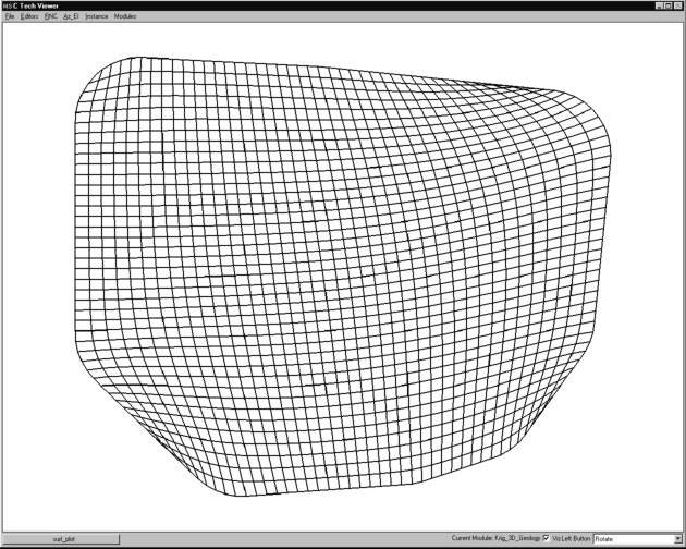
The convex hull of a set of points in two-dimensional space is the smallest convex area containing the set. In the x-y plane, the convex hull can be visualized as the shape assumed by a rubber band that has been stretched around the set and released to conform as closely as possible to it. The area defined by the convex hull offers significant advantages. Within the convex hull all parameter estimates are interpolations. The convex hull best fits the spatial extent of the data. Remember that the convex hull defines an area. That area can be gridded in many ways. EVS grids convex hull regions with quadrilaterals. Smoothing techniques are used to create a grid that has reasonably equal area cells. A two-dimensional example of a convex hull grid is shown in Figure 1.13. In this example, the domain of the model was offset by a constant amount from the theoretical convex hull. This results in rounded corners and a model region that is larger than the convex hull.

Figure 0.12 Convex Hull Grid with Offset
Adaptive gridding is the localized refinement of a grid to provide higher resolution in the areas or volumes surrounding measured sample data. Adaptive gridding or grid refinement can be accomplished in many different ways. In EVS, rectilinear, finite difference and convex hull grids can all be refined using a similar method. In two-dimensions a new node is placed precisely at the measured sample data location. Three additional nodes are placed to create a small quadrilateral cell within the cell to be refined. The corners of the small cell are connected to the corresponding corners of the cell being refined creating a total of five cells where the one previously was. The resulting nodal locations and grid connectivity must be explicitly defined.
Adaptively gridding offers many advantages. It assures that there will always be nodes at the precise coordinates of the sample data. This insures that the data minimum and maximum in the gridded model will match the sample data. It also provides greater fidelity in defining data trends in regions with high gradients. Figure 1.14 shows a two-dimensional adaptively gridded convex hull model. This model's area was also offset from the convex hull. Since each sample data point results in a refined region, and the sample points define the convex hull, the regions in each corner of the model contain adaptively gridded cells.
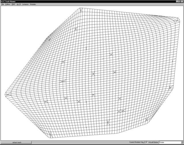
Figure 0.13 Adaptively Gridded Convex Hull Grid
Figure 1.15 is a close-up view of some refined cells near the lower right in Figure 1.14. It shows one of the special cases. If the point to be refined falls very near an existing cell edge, that edge is refined and the cells on either side of the edge are symmetrically refined. Since the edge must be broken into three segments, the cells on both sides must be affected.
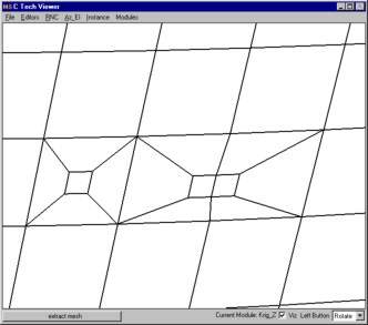
Figure 0.14 Close-up of Figure 1.14
The refinement process can also be applied to all types of 3D grids. When a sample falls in a hexahedron (hex) cell, a new much smaller hex cell is created with one of its' corners located precisely at the coordinates of the sample point. The eight corners of the small cell are connected to the corresponding corners of the parent cell. This creates 7 hex cells that fully occupy the volume of the original cell. Since the 3D-refinement process occurs internal to the volume of the model, it is more difficult to visualize the process. In order to see the refined cells, removing all cells in the grid with any nodes that were below a thresholded concentration level created Figure 1.16. By choosing the threshold properly, several of the refined cells become visible.
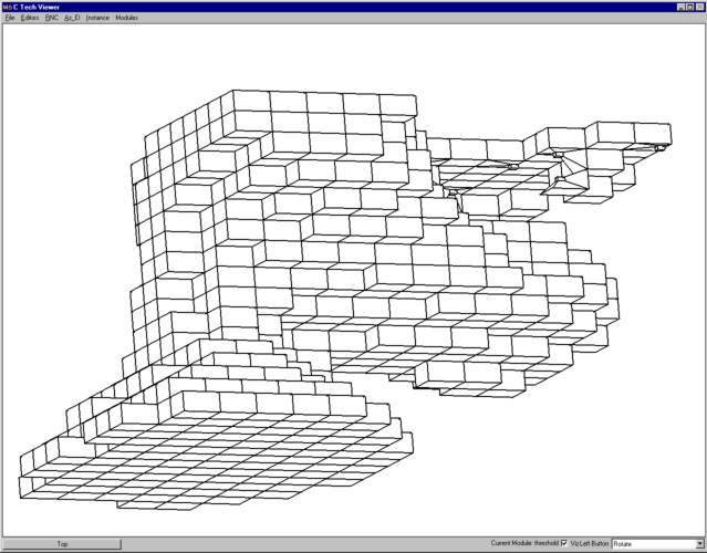
Figure 0.15 3D Adaptively Gridded Model
This figure (Figure 1.17) is an enlarged view of the upper right hand corner. It reveals the structure, relative sizes and connectivity resulting from 3D adaptive gridding.
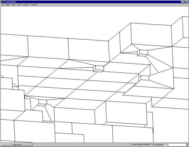
Figure 0.16 Close-up of Figure 1.16
© 1994-2018 ctech.com