Most data collection methods require drilling (or punching) a hole in the ground at a particular x-y (Easting-Northing) location. Since there is not a practical way to sample at a particular x-y-z location without drilling/boring/punching from the surface, it makes sense to determine the x-y location of sampling and collect data at multiple elevations (depths).
For that reason, we generally use Krig_2D's two dimensional kriging to determine new sampling locations. The same techniques used in this workbook are also available with Krig_3D, however. You can perform the same DrillGuide© calculations in three dimensions by using Krig_3D.
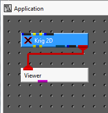
The first step is to krige your data. Begin by building the simple application shown below.
First, we'll turn OFF the "New – Reset Variables" toggle on the main window. This allows us to change values that the expert system would otherwise reset every time you run.

Open the Gridding Options window and note the "Boundary Offset:" parameter for the convex hull algorithm is 0.1. This would create a grid that was 10% larger than the convex hull of our data. Set this parameter to 0. This will force our grid to be exactly the convex hull of our data set and not offset beyond that boundary. This will ensure later, when we choose new locations, that they will be constrained to the convex hull of the original data. Sometimes you may want to have the new locations expand your site boundaries, but we will not do that for this workbook.

Close the Gridding Options and click on the "Read Data File" button:
and choose initial_soil_investigation_full_site.apdv as the analyte (e.g. chemistry) data file for this workbook.

Click on the "Accept All Current Values" button and your message console should show the following:

Please note that in the console above, this analysis was run with the demo version of EVS-PRO. There are messages here that apply specifically to the demo version. "File check passed" tells us that the file does have a valid password and will only be seen if you are running in demo mode.
Click on the "Display Settings" toggle on the main window to see the following:

Change the "Surface Vert. Scaling" parameter above to 40.0 (default is 10.0) and set your view in the Az-El Selector as shown below.

At this point, your Viewer should look like the picture below. Note that the surface has both colors and elevation that correspond to concentration. High concentration regions are green or yellow or red and correspond to mountain peaks, whereas low concentration regions are cyan or blue and correspond to valley floors.
Additionally there is a gray sphere whose purpose will be discussed in subsequent topics.

© 1994-2018 ctech.com