Visualize the Grid

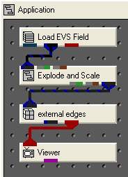
The finite-difference grid used in MODFLOW can be visualized using EVS. First, the user should create a simple application like the one shown below.

$image\wb_5_04r.jpg$

In Load_EVS_Field, choose the file multi_layer_modflow.inp in the \ctech\data\modeling folder.

Sets external_edges to have a Max Edge Angle of 0, so that all grid lines are visible.

The viewer should now appear like this:

$image\wb_5_05.jpg$

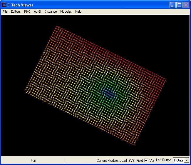
This view shows the outline of every cell in the model. The cells are currently being colored by the value of head. However, this can be changed by selecting a different Nodal Data Component in the external_edges module.

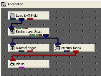
Now, let's look at the grid for this model in a different way. Modify your application to match the one below.

$image\wb_5_nt.jpg$

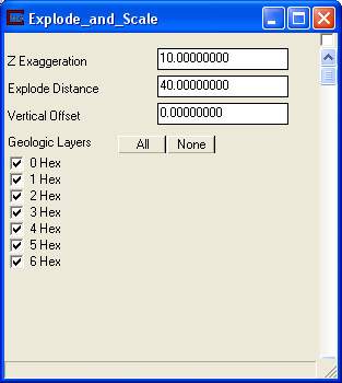
Open the main panel for Explode_and_Scale and adjust its parameters to match:

$image\wb_5_es.jpg$

Now we are going to change the modes of object display to create a hidden line view of the grid. Our layers are exaggerated and exploded and now we will color the faces the background color, and display the cell boundaries with colored lines. Since we only have one object in the Viewer (external_edges is disconnected) we could modify the properties of All Objects. We therefore don't necessarily need to use the object selector. However, if we add new modules later, they would also inherit the properties of All Objects, which is normally undesirable behavior. For this reason, we will explicitly modify the external_faces module.

In the Viewer, push the button marked "Top" in the lower left corner. This will open the Object Selector window, which should list "Top" and "external_faces". Highlight external_faces and press OK. The button in the lower left corner of the Viewer should now say "external_faces".

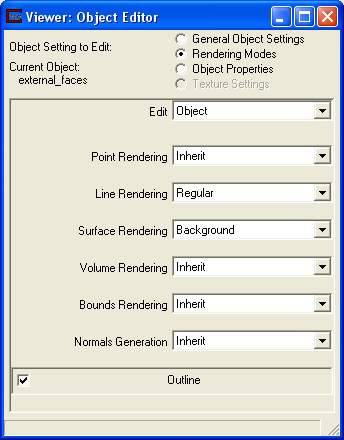
Go to Viewer, select the Editors->Object->Advanced Settings pull-down menu. Select the Rendering Modes radio button in the Viewer: Object Editor window and set the Line Rendering to Regular and Surface Rendering to Background. Your panel should look like this

$image\wb_5_ce.jpg$

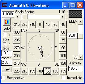
Finally let's choose to view this object differently. Open Az-El in the Viewer, and set the view to: Scale = 1.10, Elevation = 25 and Azimuth = 165, then press the multi-colored (Reset/Normalize/Center) button in the Azimuth & Elevation window in the Viewer.

$image\wb_5_az.jpg$

Your view should now be:

$image\wb_5_hg.jpg$

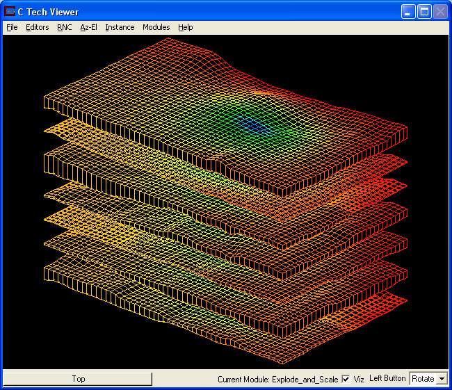
Note that we have 7 geologic layers. Each layer has only one layer of elements. This is the way the layers were modeled in MODFLOW and MT3D. Each layer has a top and bottom, but there aren't any additional (nodes) data in between. Subdividing these layers isn't necessary because EVS will interpolate for us. The outlines of the elements are colored according to Head, because this is the first data component. We could color by any (scalar) component by selecting it in external_faces.

Let's proceed to the next section and examine a few different ways to visualize head and drawdown.