EVS computes the standard deviation for each estimated point. The standard deviation is used to compute the confidence and uncertainty. The standard deviation is proportional to the square root of the sill in the variogram, since the standard deviation is computed as the square root of the variance (the second data component in MVS's KT3D module) and the variance is directly proportional to the sill.
Delete the existing application and create a simple application with Krig_2D (red port) connected to the Viewer.
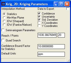
Select initial_soil_investigation_full_site.apdv. Select Accept All Current Values on Krig_2D and when it runs your Kriging Parameters should match:

Note that the Confidence BoundFactor for Statistics value is set to 10. That value will be used to determine our confidence calculations (which we will discuss very soon).
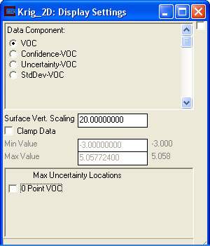
Now close the Kriging Parameters and bring up the Display Settings panel. Let's set the Surface Vert.Scaling to 20.0 and turn off the Max Uncertainty Location (since we don't want to deal with that for this topic).
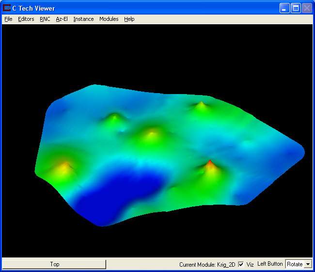
Let's also bring up the Az-El panel and set the view so that Scale = 1.10; Elevation = 45; and Azimuth = 210. Your view should now match the picture below:
Remember from Workbook 1, that this surface is colored according to concentration, and also has surface elevations (topology) which is the log of concentration times the data scaling value of 20.0.
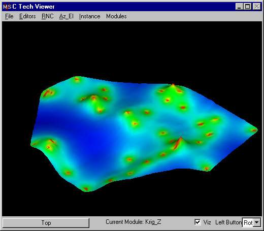
We will now select Confidence as our Data Component. This will recolor the surface, but leave the elevations unchanged. From a single picture we will be able to see confidence levels (by color) and concentration levels (by elevation).
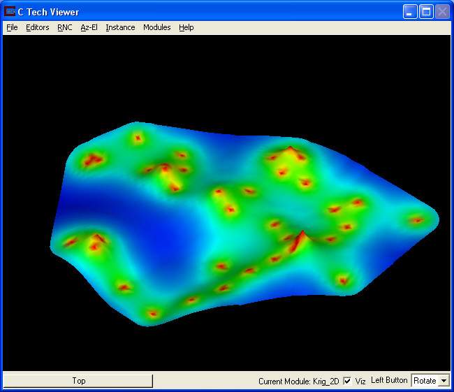
The actual Min(imum) confidence is 35.9.
Notice that the picture below has a lot of red spots. Each of these spots corresponds to a measured sample location. At every measured sample, the confidence in the estimate is 100%.
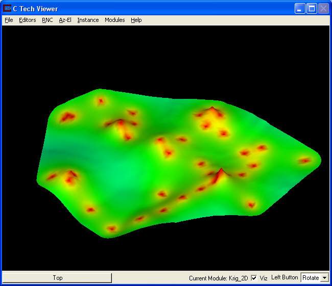
With Confidence still as our Data Component, check the toggle called ClampData. Then, set the Min Value to 0 and the Max Value to 100. This will map the blue (minimum) color to 0.0 instead of our actual data minimum, and 100 instead of our actual max (although our actual max is approximately 100). The picture will have no blue areas because our actual minimum is 35.916. This will give the following picture.
But what do we mean by Confidence? In EVS, the confidence is calculated in response to a question. For this model, the question is: What is the confidence that the predicted concentration will be within a factor of 10 of the actual concentration?
Why a "factor of ten"? Because we are working on a log10 scale, EVS took the log10 of the Conf Bound value (the value was 10, so the log is 1.0). It then compares the log concentration values and a corresponding standard deviation that was calculated for every node in our domain. For log concentrations, one unit is a factor of ten, therefore we are asking what is the probability that we will be within one unit. If you had changed the Conf Bound to 2.0, the questions would have been: What is the confidence that the predicted concentration will be within a factor of 2 of the actual concentration?
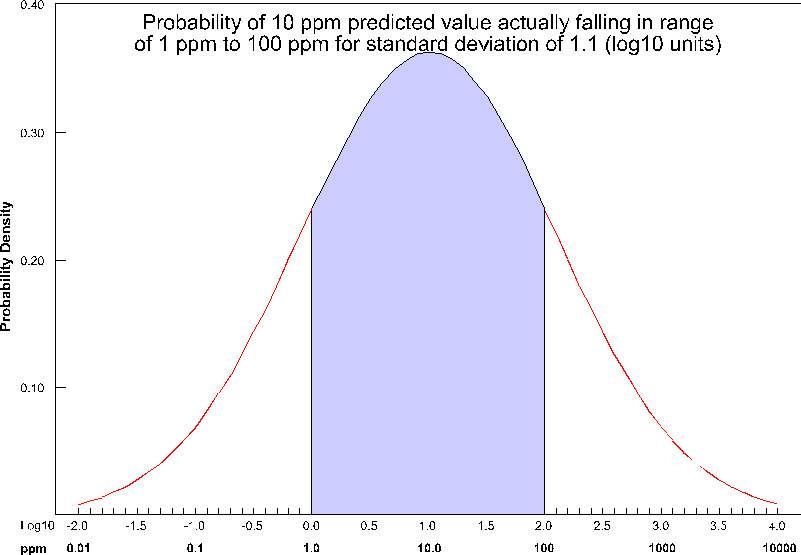
The actual calculation to determine confidence requires the standard deviation of the estimate at a node, and the Conf Bound value. The figure below shows the confidence (as the shaded area under the "bell" curve) for a Conf Bound of 10 at a node where the predicted concentration was 10 ppm (1.0 log concentration) and the standard deviation for this point was 1.1 (in log10 units). For this example, the confidence would be ~64%, which means that 64% of the time, the value would lie in the shaded region.
© 1994-2018 ctech.com