Three dimensional parameter estimation using EVS's kriging modules is straightforward and provides powerful capabilities to assess complex underground distributions of chemicals, ore bodies or other geologic properties (head, porosity, conductivity, etc.). The relevant modules specific to three dimensional kriging are:
1) Krig_3D
2) Krig_3D_Geology
3) Spline_Geology
4) Indicator_Geology
The second and third modules provide inputs to Krig_3D to allow mapping of chemical concentrations to geologic structures. A very large number of other EVS modules provide useful and important capabilities related to visualization and analysis of the output of Krig_3D, but their functionality is not restricted to its output. The Indicator_Geology module performs 3D kriging of geologic data.
A Simple Network for 3D Kriging
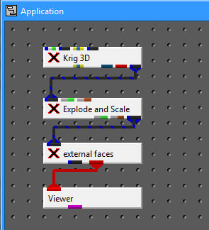
Using the methods covered in Workbook 1 and 2, instance the modules and connect them to form the network shown in the figure below.
In this network, Krig_3D produces the model, Explode_and_Scale allows us to exaggerate the "Z" coordinate (and later to explode layers) and external_faces allows us to visualize the external surfaces of the model.
Before we run this network, let's modify a few of the parameters. Begin by selecting Krig_3D from the Modules pull-down menu to reveal the Krig_3D Main menu shown below.

SelectData Processing so that we may change a few values.
Now modify Post-ClipMax: in the Data Processing window to be 1.000000e+003 (1000).
Close only the Data Postprocessing subwindow (we'll want to look at the Gridding Options after the module runs) and click on the Read Data File button to reveal the file browser shown below.

Select the file shown (initial_soil_investigation_subsite.apdv) by double clicking, or by clicking once and then selecting Open.
Click on the "Accept All Current Values" button and the network will run.
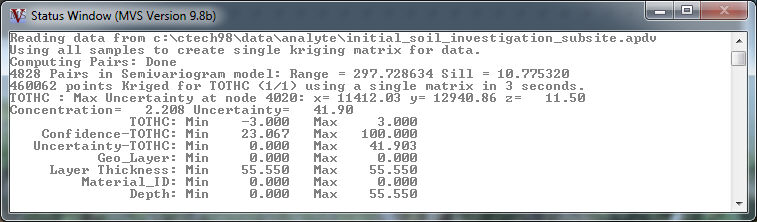
As Krig_3D runs, it will print status messages to the console. These include time to completion estimates. On most modern computers, this network will run almost instantaneously. When it is complete, the console will show the following messages.
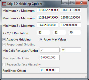
If we now open Gridding Options, those parameters which were initially 0.00 (zero default values) have been updated. The Min/Max X-Y-Z values have been set to the extents of the analyte (e.g. chemistry) file. Note that the maximum Z value is now determined using the Top of boring elevation from the highest boring, rather than the elevation of the highest sample. It is nearly always best to use geologic input, however when there is none, this will give you a grid that goes to the highest ground surface elevation.
The updated gridding values are shown in the figure below.
Other values which were initially 0.00 (zero default values) such as Reach have also been set in Kriging Parameters. For detailed descriptions of all of the parameters in Krig_3D (or any other EVS module) please refer to the Module Libraries references in the manual or on-line help....OR...select any module, click the right mouse button and choose help.
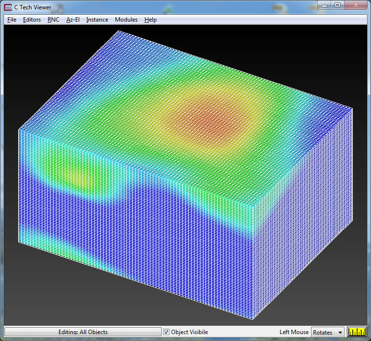
At this point the network has run to completion and a visualization of the external faces of the domain has been produced. We now see a top view of the model in the Viewer. Choose Az-EL and set the Elevation to 35 degrees, Scale to 0.90 and click on the 150 degree Azimuth button. At this point your Viewer should look like this:

Notice that the domain is a flat-surfaced "brick". Since no geology data was used to produce the output, the extents of the domain were determined by the extents of the input file.
If we want to see the grid used to create this model, go to the Viewer pull down menus and select Editors->Object->Advanced Settings

and in the ObjectSetting to Edit: select Rendering Modes. Change Line_Rendering to Regular. This should display the picture below.
Before proceeding to the next topic, reset Line_Rendering (Object Editor) to inherit and close the Viewer:Object Editor window.
© 1994-2018 ctech.com