

This is an EVS-PRO & MVS module only.
Indicator_Geology is an alternative geologic modeling concept that uses the indicator method for assigning each cell’s lithologic material as defined in a pregeology (.pgf) file, to cells in a 3D volumetric grid.
General Module Function
Module Input Ports
Indicator_Geology has an Orange-Blue-Yellow input port that can receive the geology file name and a (gray-magenta) port outputs the refine distance to Pre_Geology.
Indicator_Geology has three input ports.
The leftmost (blue/white/green) port can accept a data field from Krig_3D_Geology to constrain indicator kriging between two topographic surfaces.
The second (Orange-Blue-Yellow) port receives the pre-geology file name.
The third port (gray-magenta) port receives the refine distance.
Module Output Ports
Indicator_Geology has three output ports.
The first (Orange-Blue-Yellow) port supplies the pre-geology file name to Pre_Geology.
The second (gray-magenta) port outputs the refine distance to Pre_Geology.
The third port (blue-black) is the primary output field containing cell data representing geologic materials.
Module Status: Interruptible
This module's computational processes can be terminated (interrupted) using the "C Tech" icon in the Windows Notification Area (aka System Tray) in the lower right corner of your desktop. If you hover over the icon, it will tell you the status of the module and expected completion time. Double-Right-Clicking will terminate the process. Note that if you do stop any process, the output of the module is corrupted and any downstream module's results are not usable. You will need to re-run the module.

Module Control Panel
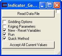
The control panel of Indicator_Geology is shown in the figure above. The ReadDataFile button opens the File Browser panel shown in the figure below.
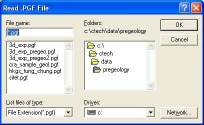
The file browser is a standard window browser that allows the user to specify the directory in which the files reside, and the extension used to filter the displayed available file names. For Indicator_Geology, the only file extension is .pgf. The format of .pgf files is described in the pgf_file_format Help topic.
The "Run" toggle controls whether the module will run when applications are loaded or data changes. When this is on, the module runs when applications are loaded or the "Accept" button is pushed. When it is off, the module will not run.
The Quick Method toggle removes Semivariogram Parameters as an option and utilizes a substantially simplified algorithm for indicator kriging. In many cases the results are comparable to the more rigorous method and it is always much quicker.
Note: The "new" toggle on the main panel (on by default) resets all expert system calculated variables to zero before each run. This allows multiple calculations to be performed without tedious manual resetting of these variables. To change an expert system calculated variable, the toggle must be off.

1) The Quick Method assigns the lithologic material cell data based on the nearest lithologic material (in anisotropic space) to your PGF borings. This is now done based on the cell center (coordinates) and an enhanced refinement scheme for the PGF borings. In general the Quick Methodshould not be used for final results.
2)For the morerigorous probabilistic approach to geologic indicator kriging, the probability for each material is computed for each cell center of your grid. The material with the highest probability is assigned to the cell. All of the individual material probabilities are provided as additional cell data components. This will allow you to identify regions where the material assignment is somewhat ambiguous. Needless to say, this approach is much slower (especially with many materials), but often yields superior results and interesting insights.
Module Parameter Subpanels
Indicator_Geology has two subpanels which allow the user to set the parameters used for Gridding Options and setting the KrigingParameters. Clicking on either the check boxes next to the subpanel names, or on the names themselves will bring up the subpanel data entry screens.

The Gridding Options subpanel of Indicator_Geology is shown in the figure above.
The Minimum X, Maximum X, Minimum Y, Maximum Y, Minimum Z and Maximum Z parameters allow the user to define the horizontal and vertical domain within the data set in which kriging of the parameter distribution will be completed. A value of 0 is the default for these parameters, which results in a model domain that is defined by the rectilinear bounds of the entire data set when the module is run. Indicator_Geology utilizes a model domain that is bounded by the limits of the data set, unless the user specifies a different domain by setting the Min and Max Values for X,Y, and Z, or it is passed a model (or finite-difference) domain from Krig_3D_Geology. Utilizing the default extents effectively minimizes the extrapolation of parameters within the model to that area which is enclosed by the measured data points. Note that when a geologic model domain is passed to Indicator_Geology, the kriging domain is restricted to that domain regardless of what X, Y, or Z values are set in the Indicator_Geology inputs. The geologic model domain can be bounded by the convex hull of the data set, or by some specified offset (see discussion in Krig_3D_Geology). If the user is uncertain of the X, Y and Z limits of the data domain, the module should be run with the default 0 values, and upon completion of execution, the values in the X, Y, and Z input fields will be the min and max values of these parameters in the data set. The File Statistics module can also be used to investigate the limits and distribution of values in the input data set, and the statistics module can be used to output the distribution of values in the kriged model.
The X / Y / Z Resolution parameters specify the number of grid nodes that will be included within the model domain. If Indicator_Geology is being passed a model domain from Krig_3D_Geology, then the x-y values are not used . The number of grid elements along any axis of the model is simply the axis Res value minus one, as every element has two bounding nodes along an axis. The default value for the X and Y Res parameters is 41, and the default value for the Z Res is 35. However, the user can specify any number desired, up to the limit of available memory resources in the computer and run time limitations imposed by the patience of the user.
If geologic layers are being passed to Indicator_Geology, then the number of nodes specified in Z Res will be distributed over the geologic layers in a manner that is approximately proportional to the fractional thickness of each layer relative to the total thickness of the geologic domain. However, in all cases, at least three layers of nodes (2 layers of elements) of the Indicator_Geology domain will be placed in each geologic layer.
Reverse Surface Hierarchy - This toggle determines whether the surfaces will define layers in a normal (top to bottom) manner or reversed (if on). This topic is discussed in more detail in Workbook 12.
Minimum Layer Thickness forces layers thinner than the specified value to have a minimum thickness and therefore not pinch-out completely.
The Rectilinear Offset parameter is used to create an automatically generated rectilinear domain which is larger than the input data set by a user input percentage along all three axes. If 10% (0.1 default value) is used, the limits will be offset by 5% on all 6 sides of the rectilinear volume.

The Kriging Parameters subpanel of Indicator_Geology is shown in the figure above.
The Reach input field defines the radial distance (in user units) from any given model node that the kriging module will look for data points to be included in the estimation of the model parameter at that node. The default value of reach is 0, which results in the module calculating a reach value which is approximately two-thirds of the longest distance between any two data points in the data set.
The Points parameter defines the maximum number of data points (within the specified reach) that will be considered for the parameter estimation at a model node. The default value for points is 20, which generally provides reasonably smooth modeled parameter distributions. The effects of decreasing and increasing the values for reach and points on the model output are somewhat similar, but for different reasons. If the data have a fairly even spatial distribution throughout the domain, then increasing these values will generally include more of the input data points that will be used to krige the value for a given model node, and thus will result in smoother modeled data distributions. Decreasing the values of reach and points (in an evenly distributed data set) results in fewer input data points being used to calculate the parameter estimates at a given model node, and result in modeled distributions with greater variations across smaller areas.
The user should consider both the spatial distribution and the range of values in the input data set when deciding upon values for the reach and points parameters. If the specified reach is too small to allow the kriging module to locate at least one point within the search area, then no kriging will be completed and the following error will be printed to the Status Window:
Matrix Singular. Increase REACH. Your reach is so small that no samples fall within the search radius.
If the user specifies a large number of points (that are within the specified reach), then the output will be smoother, but the execution time for the kriging can increase significantly. By posting the input data using the post_samples module, and looking at the characteristics of the resulting kriged data using the Statistics module, the user can quickly analyze the characteristics and distribution of the kriging output for a given set of parameters, and test the effects of changing the kriging parameter values.
The Octant Search toggle changes the method by which data sample points are selected for inclusion in the kriging matrix. If this is on, the "Points" parameter switches to "Max Points in Octant". Searching is performed for each of the eight Octants surrounding the point to be kriged. Within each octant a maximum number of points (up to one-fourth of the total points) are selected. Then, points are taken sequentially from each octant up to the maximum number of total points or until all octant’s points have been used. The panel display changes when this option is selected as shown above. Octant Search is applicable for the Statistics and Min-Max Plume kriging modes. Octant Search cannot be used with the Quick Method.
Understanding the Refine Dist(ance) parameter requires an understanding of the basics of indicator kriging with a .PGF file as input. Since a PGF file has only a single point defining the bottom of intervals of a specific material, it is necessary to create an intermediate dataset that is used for the actual kriging. Since each interval represents a line segment with constant material characteristics, we approximate it by refining the interval into a set of points. The spacing between these points affects accuracy. Each segment will receive at least two points near the end points of the interval, but longer segments will broken up into segments no larger than the refine distance. Setting this value too small will result in much greater run times, as well as requiring higher values for the points parameter. Setting this value too large can create artificial inaccuracies in the prediction because the center of the intervals can have a lack of sample points, causing points in other borings to appear closer. If you leave the default setting of 0.00 for this parameter the expert system determines the spacing for you by searching the original PGF file for the shortest segment in any boring. The calculated refine distance will be twice the shortest segment length or one half the height of the first cell in the grid, whichever is larger. This tends to give reasonable results with most datasets. You can also use the Pre_Geology module to visualize the refined points directly by setting its refine distance parameter to be the same as the computed one in Indicator_Geology.
Since a PGF file has only a single point defining the bottom of intervals of a specific material, it is necessary to create an intermediate dataset that is used for the actual kriging. Since each interval represents a line segment with constant material characteristics, we approximate it by refining the interval into a set of points. The spacing between these points affects accuracy. If you leave the default setting of 0.00 for this parameter the expert system determines the spacing for you by searching the original PGF file for the shortest segment. This minimum distance will receive two points surrounding the center of the interval and longer segments will receive many more. Setting this value too small will result in much greater run times.
The Horiz./Vert. Anisotropy Ratio parameter allows the user to consider the effects of anisotropy in the conductivity of soil matrices to fluid flow. In most cases, geologic materials are deposited with platy clay minerals oriented horizontally, and thus flow of water in both the saturated and unsaturated zone can be slower in the vertical direction than in the horizontal direction. Also, ore deposition can occur along horizontal or vertical fault or fracture systems. Chemical constituents being transported with flowing fluids may therefore show a larger degree of spreading in one or the other direction. The Horiz./Vert. Anisotropy Ratio basically tells the kriging algorithm what multiplication factor should be used to apply biased weighting on data points in horizontal and vertical directions away from a given model node. The default value is 10, which allows data points in a horizontal direction away from a model node to influence the kriged value at that node 10 times more than data points an equal distance away in a vertical direction. However, the user can specify any positive number with a magnitude up to 100,000. When the property being modeled is not related to fluid flow or other processes that might be affected by matrix anisotropy, then this parameter should be set to 1.
General Discussion of Geologic Indicator Kriging vs. Hierarchical Geologic Modeling
C Tech's original method for 3D geologic modeling utilizes one of two different ASCII file formats (.geo and .gmf) which contain "interpreted" geologic information. These two file formats both describe points on each geologic surface (ground surface and bottom of each geologic layer), based on the assumption of a geologic hierarchy.
The easiest way to describe geologic hierarchy is with an example. Consider the example below of a clay lens in sand with gravel below. Some borings will see only sand above the gravel, while others will reveal an upper sand, clay, and lower sand.
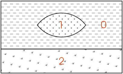
The geologic hierarchy for this site will be upper sand, clay, lower sand, and gravel. This requires that the borings with only sand (above the gravel) be described as upper sand, clay, and lower sand, with the clay described as being zero thickness. For this simple example, determining the hierarchy is straightforward. For some sites (as will be discussed later) it is very difficult or even impossible.
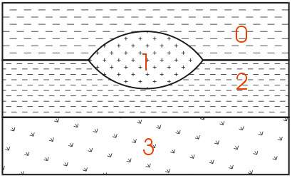
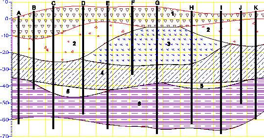
For those sites that can be described using the above method, it remains the best approach for building a 3D geologic model. Each layer has smooth boundaries and the layers (by nature of hierarchy) can be exploded apart to reveal the individual layer surface features. In the above example, the numbers represent the layer numbers for this site (even though layers 0 and 2 are both sand). Two examples of much more complex sites that are best described by this original approach are shown below.
Geologic Example: Sedimentary Layers and Lenses
Geology Example & Figure: Outcrop of Dipping Strata
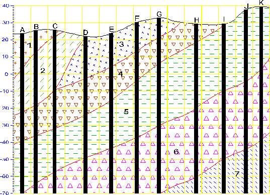
EVS is not limited to sedimentary layers or lenses. The figure below shows a cross-section through an outcrop of dipping geologic strata. EVS can easily model the layers truncating on the top ground surface.
However, many sites have geologic structures (plutons, karst geology, sand channels, etc.) that do not lend themselves to description within the context of hierarchical layers. For these sites, Geologic Indicator Kriging (GIK) offers the ability to build extremely complex models with a minimum of effort (and virtually no interpretation) on the part of the geologist. GIK can also be a useful check of geologic hierarchies developed for sites that do lend themselves to a model based upon hierarchical layers.
GIK uses raw, uninterpreted 3D borings logs as the input file. The .pgf (pre-geology file) format is used to represent these logs. PGF files contain descriptions of each boring with x,y, & z coordinates for ground surface and the bottom of each observed geologic unit. Consecutive integer values (e.g. 0 through n-1, for n total observed units in the site) are used to describe each material observed in the entire site.
NOTE: It is important to start your material ID numbering at zero (0) instead of 1.
Usually, materials are numbered based upon a logical classification (such as porosity or particle size), however the numbering can be arbitrary as long as the numbers are consecutive (don’t leave numbers out of the sequence). For the example given above, we could number the materials as shown in the figure below (even though it is not a numbering sequence based on porosity or particle size).
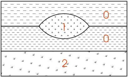
For a .pgf file, borings that do not see the clay (material 2 in the figure) would not need to consider the sand as being divided into upper and lower. Rather, every boring is merely a simple ASCII representation of the raw borings logs. The only interpretation involves classification of the observed soil types in each boring and assigning an associated numbering scheme.
As an example, we have taken the Site T geologic data and created a model using both methods. This is a moderately complex site with geology that can be represented with hierarchical layering. However the complexity at this site does require a significant amount of interpretation (by a geologist or analyst) that lends a subjective element to the resulting model. The figure below shows the .pgf file for this site representing 5 unique materials.
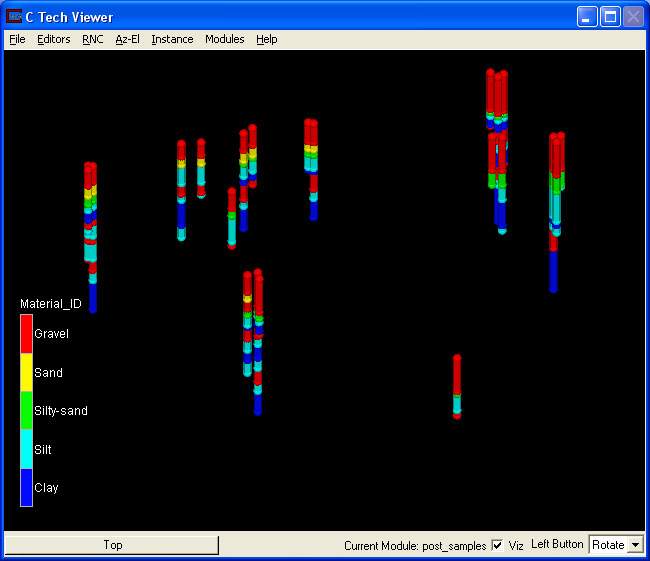
Note that there is a significant difference in the depths of some of the borings. Most notably, AW-3 (right foreground) is much shallower than the rest and is located quite a distance from any neighboring borings. With both techniques, extrapolation of the geology to the region below AW-3 will be low confidence and we expect that the two methods (Geologic Hierarchy and Geologic Indicator Kriging) will yield different results.
However both techniques should (and will) result in the same layering in the vicinity of the borings. This is a common theme in EVS for both geology and chemistry data. EVS will honor your measured data.
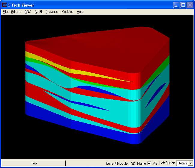
The figure below is the geologic hierarchy model for Site T. Note that the layers have relatively smooth boundaries and transitions (in thickness) from one boring to the next. Also note that the extrapolated geology below AW-3 is a logical extension from the neighboring borings. Please remember that a significant effort was required to interpret the .pgf file and create an interpreted geologic data file (.gmf file) that was used to create this model.
This next figure shows the model produced using GIK. The most notable difference is that the boundaries between layers are blocky. This is due to the totally different approach. With GIK, a default grid is created (per a user-specified fineness). This grid can be (and is in this case) defined between two geologic surfaces (e.g. ground surface and the bottom of gravel). The finer the grid (especially in the vertical direction) the more accurate the representation. GIK assigns the most probable material to each CELL in the model. The assignment to a cell is a significant distinction as compared with all other interpolation performed in EVS/MVS. If geologic data were assigned to nodes (vs. cells), in areas where there is a transition between two non-sequential material id’s, colors would be interpolated between them that would correspond to intermediate materials. Using the cell data paradigm, we can have regions that transition from Clay to Gravel without seeing any other materials interpolated in between.
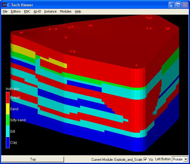
Also note that regions produced with GIK can have vertical transitions and folds. It is not encumbered by the layered approach of geologic hierarchy.
In conclusion, for this site, the decision of which approach is best is unclear. The greatest differences in the models are in areas where there is a lack of data. Ultimately a geologist familiar with the conditions should make that determination. For other sites, the choice between the two approaches is often quite obvious (especially if interpretation is too difficult).
© 1994-2018 ctech.com