

General Module Function
The Krig_3D_Geology module uses data in .geo files and .gmf files to model the surfaces of geologic layers that will provide the geologic framework for three-dimensional geologic modeling and parameter estimation. Krig_3D_Geology creates layers of quadrilateral (4 node) elements in which each node is assigned the kriged elevation for the specific geologic surface at that point in space. The output of Krig_3D_Geology is a data field that can be sent to the Krig 3D and 3D Geology Map modules where the quadrilateral elements are connected to the element nodes in adjacent geologic surfaces to create layers of hexahedral (8-node) elements. The output of Krig_3D_Geology can also be sent to the Geologic Surface module which will allow visualization of the individual layers of quadrilateral elements (the surfaces) that comprise the surface layer and the bottoms of each geologic layer. Krig_3D_Geology has the capability to produce layer surfaces within the convex hull of the data domain, within a rectilinear domain with equally spaced nodes, or within a rectilinear domain with specified internodal distances such as a finite-difference model grid. The finite-difference gridding capabilities allows the user to visually design a grid with variable spacing, and then krige the geologic layer elevations directly to the finite difference grid nodes. This functionality facilitates setup of finite difference and or hexahedral element finite element model input files. Krig_3D_Geology also provides geologic surface definitions to the post_samples module to allow exploding of boreholes and samples by geologic layer.
Note: Krig_3D_Geology has the ability to read .apdv, .aidv and .pgf file to create a single geologic layer model. This was not done as a preferred alternative to creating/representing your valid site geology. However, most sites have some ground surface topography variation. If Krig_3D is used without geology input, the resulting output will have flat top and bottom surfaces. The flat top surface may be below or above the actual ground surface at various locations. This can result in plume volumes that are inaccurate.
When a .apdv or .pgf is read by Krig_3D_Geology or Spline_Geology the files are interpreted as geology as follows:
1) If Top of boring elevations are provided in the file, these values are used to create the ground surface.
2) If Top of boring elevations are not provide in the file, the elevations of the highest sample in each boring are used to create the ground surface.
3) The bottom surface is created as a flat surface slightly below the lowest sample in the file. The elevation of the surface is computed by taking the lowest sample and subtracting 5% of the total z-extent of the samples.
When reading these files, you will get a single layer which goes to either the Top column (if it exists) otherwise, the top sample in each boring, and 5% below the lowest sample in the file (flat bottom). This allows you to create a convex hull around data without having geology info. It also provide a topographic top surfaces if your analyte (e.g. chemistry) or PGF file has Tops (grounds surface elevations). Also nice for doing indicator kriging (since a single, well-defined pgf can give you an entire indicator model now). Be aware that if Top is specified, but all values are exactly 0.0, the top sample elevation for each boring will be used.
Module Input Ports
Krig_3D_Geology has an Orange-Blue-Orange input port that can receive the geology file name.
Module Output Ports
Krig_3D_Geology has six output ports.
1) Read_geo_data_file (Orange-Blue-Orange) : Supplies the geology file name.
2) Vistas Group (blue-magenta-blue-magenta) : Provides input to the Geology_to_Vistas module.
3) Geology Material Names (Brown-Grey-Light Brown-Beige) : Provides geologic material information for the Legend module.
4) status_out(blue/green) : Outputs a string containing status updates while the module is running.
5) output0 (blue-white-green) : The primary output field. The primary output field port can be connected to the Krig_3D, 3D_Geology Map, and Geologic Surface modules.
6) Grid_out (red) : Outputs a renderable geometry of a finite difference grid.
Module Status: Interruptible
This module's computational processes can be terminated (interrupted) using the "C Tech" icon in the Windows Notification Area (aka System Tray) in the lower right corner of your desktop. If you hover over the icon, it will tell you the status of the module and expected completion time. Double-Right-Clicking will terminate the process. Note that if you do stop any process, the output of the module is corrupted and any downstream module's results are not usable. You will need to re-run the module.

Module Control Panel
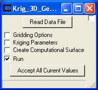
The control panel of Krig_3D_Geology is shown in the figure above. The ReadDataFile button opens the File Browser panel shown in the figure below.
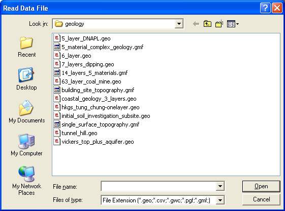
The file browser is a standard window browser that allows the user to specify the directory in which the files reside, and the extension used to filter the displayed available file names. For Krig_3D_Geology, the default file extension is .geo, .apdv, .aidv, .pgf, or .gmf. The format of .geo files is described in the geo_file_format Help topic. The format of .gmf files is described in the gmf_file_format Help topic.
Note that this module will begin running only when a file is selected and the Accept All Current Values button is pushed. However, if a finite difference grid domain is to be setup for the kriging, then a geology file should not be selected until the grid domain has been setup.
The "Run" toggle controls whether the module will run when applications are loaded or data changes. When this is on, the module runs when applications are loaded or the "Accept" button is pushed. When it is off, the module will not run.
Both .geo and .gmf geology files support inclusion of parameters to specify geologic layer material number. Within EVS, layers are numbered beginning with the top layer as zero. Previously, there was no other parameter associated specifically with layers. Now, each layer can be assigned a material number. This allows for specifying layer material independent of layer number.
Module Parameter Subpanels
Krig_3D_Geology has three subpanels, which allow the user to set the parameters used for creating the kriging grid, the semivariogram production, and for creating compututational surfaces. Clicking on either the check boxes next to the subpanel names, or on the names themselves will bring up the subpanel data entry screens. Note that the subpanels have to be closed by clicking on the box in the Module Control Panel.
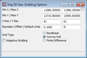
The Gridding Options subpanel of Krig_3D_Geology is shown above.
Although it is at the bottom of the subpanel, the first option that should be set by the user is Grid Type, as this will determine the nature of the domain that will be kriged. The Rectilinear option is used when the user wishes to produce a model that contains estimated values everywhere inside a user specified rectangular domain. The Convex Hull Boundary Option is used when the user wishes to produce a model that can have an irregular boundary that is defined by the distribution of measured data points. The Convex Hull of a data set can be thought of as the domain that would be outlined by stretching a rubber band around the external data points in the data set. The Convex Hull boundary option effectively minimizes the extrapolation of parameters within the model to that area which is enclosed by the measured data points. The Finite Difference domain allows the user to krige the elevations of the geologic layers directly to the finite difference grid node locations that were setup in the control panel of Krig_3D_Geology. Note that the finite difference grid must be designed and displayed before the user selects a .geo file and clicks the Accept all Current Values button.
Adaptive Gridding causes the grid nodes to be shifted up to 30% of a cell width to cause the nodes to align with your input data values. By having grid node coincident with surface points, the grid will exactly honor the surface at that location. This help maintain accuracy with coarser grids.
The Min X, Max X, Min Yand Max Y inputs allow the user to define the horizontal domain within the data set in which kriging of the geologic surfaces will be completed. The Min and Max values are only used when the Rectilinear Option is selected. The Min (x-y) values are also used to set the origin for the Finite Difference Grid Type option. A value of 0 is the default for these parameters, which results in a model domain that is defined by the entire data set when the module is run. When kriging within a finite difference domain, the Min (x-y) values are used to set the origin (lower left hand corner before grid rotation). If the user is uncertain of the X and Y limits of the data domain, the module should be run with the default 0 values, and upon completion of execution, the values in the X and Y input fields will be the min and max values of X and Y in the data set. Alternatively, the File_Statistics module can be used to examine the data characteristics. There is no specification of the Z grid dimensions, as Krig_3D_Geology outputs 2-D surfaces of each geologic interface. The modules that use the output of Krig_3D_Geology define the Z grid dimensions as specified by the user in those modules.
The X Res and Y Res parameters specify the number of grid nodes that will be included within the model domain. The number of grid elements along either axis of the model is simply the X Res or Y Res value minus one, as every element has two bounding nodes. The default value for these parameters is 41, but the user can specify any number desired, up to the limit of available memory resources in the computer and run time limitations imposed by the patience of the user. The robust kriging algorithms in EVS generally produce reasonable modeled distributions with a fewer number of grid nodes than the user may be used to, so the recommended procedure for setting the X and Y Res parameters is to start with less, and then increase the value until an acceptable model fidelity is obtained.
The Boundary Offset parameter sets the distance that the convex hull for the kriging domain will be set outside of the actual convex hull of the data. This parameter allows the user to specify the distance outside of the actual data in which the parameter values will be extrapolated. The distance is a percentage of the diagonal extent in the X-Y plane. The default is 0.10 (10%). For example: if data extent is 100 in x and 100 in y, diagonal distance is 144. It will make the convex hull offset 14.4 total by offsetting 7.2 on all sides. This eliminates dangerously large offsets when data extent is small.
The Default Units parameter allows the user to set the coordinate units of the model if the file being read does not contain them. If the file does contain coordinate units, this parameter is ignored.
To set up a finite difference grid, the Gridding options checkbox should be checed and the Finite Difference Grid Type should be selected, which will bring up the X and Y check boxes, and the Angle data input field. The angle input field allows the user to specify an angle in degrees counter-clockwise from true north that the resulting grid will be rotated. The finite difference grid corresponding to the input parameters can be visualized at any time by clicking the Accept All Current Values button (before a .geo file has been specified in the file browser). The Finite Difference Gridding subpanels for X and Y allow the user to constrain the modeled domain to be within the finite difference grid setup using the Krig_3D_Geology control panel. Note the X and Y values specified in these subpanels override any other specified values for Min and Max X and Y in the Gridding Options. Clicking on the X or Y subpanels in finite difference gridding brings up a subpanel similar to the one shown in the figure below.
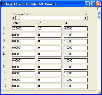
The first parameter is a slider to specify the total Number of Steps (grid regions). There is no limit to the number of steps (regions) and each region can any number of elements (cells) and can have constant size cells, decreasing (Cx < 1.0) or increasing (Cx>1.0).
The user builds the finite difference model grid by specifying the distance between the first and second grid nodes (or the element width) in the Del X input field. The number of additional nodes to be placed at this spacing is then specified in the Xr (standing for "X repeat") input field. If a gradually varying node spacing is desired between the number of nodes specified in Xr, then a multiplication factor is specified in the Cx (standing for "Change X") input field. Values greater than 1.0 create an increasing element size, and values less than 1.0 create diminishing element sizes. The grid design process is identical for the Y grid panel. These panels allow the user to quickly design and visualize a rectilinear model grid.
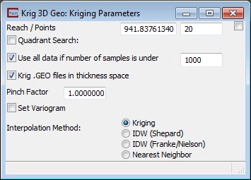
The KrigingParameters subpanel of Krig_3D_Geology is shown in the figure above.
The Reach input field defines the radial distance ( in user units) from any given model node that the kriging module will look for data points to be included in the estimation of the model parameter at that node. The default value of reach is 0, which results in the module calculating a reach value, which is approximately two-thirds of the longest distance between any two data points in the data set.
The Points parameter defines the maximum number of data points (within the specified reach) that will be considered for the parameter estimation at a model node. The default value for points is 20, which generally provides reasonably smooth modeled parameter distributions. The effects of decreasing and increasing the values for reach and points on the model output are somewhat similar, but for different reasons. If the data have a fairly even spatial distribution throughout the domain, then increasing these values will generally include more of the input data points that will be used to krige the value for a given model node, and thus will result in smoother modeled data distributions.
Decreasing the values of reach and points (in an evenly distributed data set) results in fewer input data points being used to calculate the parameter estimates at a given model node, and result in modeled distributions with greater variations across smaller areas. The user should consider both the spatial distribution and the range of values in the input data set when deciding upon values for the reach and points parameters. If the specified reach is too small to allow the kriging module to locate at least one point within the search area, then no kriging will be completed at that model node, the nodal value will be set to 0, and the confidence level will be set to <0.1%. Note that this nodal value is generally inappropriate, and the regions of the model receiving the 0 values should be subsetted out of the by using an plume_volume module with a confidence isocomponent of 1%. If the user specifies a large number of points (that are within the specified reach), then the output will be smoother, but the execution time for the kriging can increase significantly. By posting the input data using the post_samples module, and looking at the characteristics of the resulting kriged data using the Statistics module, the user can quickly analyze the characteristics and distribution of the kriging output for a given set of parameters, and test the effects of changing the kriging parameter values.
The Quadrant Search toggle changes the method by which data sample points are selected for inclusion in the kriging matrix. If this is on, the "Points" parameter switches to "Max Points in Quadrant". Searching is performed for each of the four quadrants surrounding the point to be kriged. Within each quadrant a maximum number of points (up to one-half of the total points) are selected. Then, points are taken sequentially from each quadrant up to the maximum number of total points or until all quadrant’s points have been used. The panel display changes when this option is selected as shown above.
The type-in value for Use all data if number of samples is under is off by default, but this option gives the smoothest surfaces since all data is used for the kriging process. Sometimes using all points results in faster computation since only one (large) kriging matrix must be solved.
The Krig .GEO files in thickness space toggle off causes GEO files to be kriged like GMF files. Each surface get kriged independently of the other surface instead of being kriged in thickness space. This only applies to GEO files without the $W/$G flags.
The Pinch Factor parameter provides the ability to control where pinching occurs between positive thicknesses and borings having the pinch flag. It defaults to 1.0 which causes pinching to occur approximately half-way between positive thicknesses and borings having the pinch flag. When older applications created before version 9.5 are loaded they will have a value of 0.0 for backwards compatibility.
Kriging (this is the default and the only option available up to Version 9.0)
IDW (Shepard)
IDW (Franke/Nielson)
Nearest Neighbor
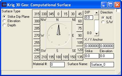
The Create Computational Surface panel is shown above. This method will create three different types of surfaces based upon the created grid. A file is required for a computational surface to be created. The first step is to create the desired grid using the Gridding Options subpanel discussed above.
The Surface Type radio box is the next step. There are three different types of surfaces that can be created. The Strike Dip Plane option consists of a single surface that can be rotated to match both strike and dip values. This option also requires an 3D coordinate point to center the rotation plane. This coordinate point is entered into the X / Y Anchor fields as well as the Elevation field. A MaterialNumber and Surface Name can also be entered for this computed surface.
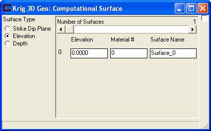
The Elevation suface parameters can be seen in the image above. This surface type will create any number of surfaces all with the same X, Y coordinates created by the gridding options, but at set elevations. The Material Number and the Surface Name can be set for each surface.
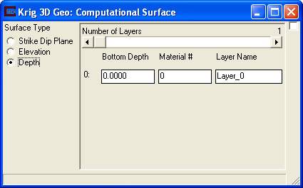
The Depth surface paramets can be seen above. This method will Krige the selected file onto the grid created using the gridding options. It will then create any number of layers at specified depths below the top surface. The Material Number and Layer Name can be set for each layer.
Explanations of the various parameter settings and their effects on the visualization are provided in Workbook 2.
© 1994-2018 ctech.com