post_samples

(This module has some features available only in EVS PRO and MVS)

General Module Function

The post_samples module is used to visualize:

Sampling locations and the values of the properties in .apdv files
The lithology specified in a .geo file
The location and values of well screens in a .aidv file

along with a representation of the borings from which the samples/data were collected. The post_samples module has the capability to process property values to make the posted data values consistent with data used in kriging modules. Data can be represented as spheres or any user specified glyph. The sampling locations may be colored and sized according to the magnitude of the property value, and labels can be applied to the sampling locations with several different options.

Each sampling location can probed for data by holding the alt button and left-clicking on the sample location.

The post_samples module can also represent downhole geophysical logs or Cone Penetration Test (CPT) logs with colored and sized tube diameters according to the magnitude of the data. It can display nonvertical borings and data values collected along their length, and can also explode borings and sample locations to show their correct position within exploded geologic layering.

When used to read geology files, post_samples will place surface indicators at the top (ground) surface and the bottom of each geologic layer that are colored according to the layer they depict. When a geology file (.geo or .gmf) is exploded without using geologic surface input from Krig_3D_Geology (or Spline_Geology) there will be surface indicators at the top and bottom of each layer. You may color the borings by lithology.

Module Input Ports

(For EVS PRO and MVS)

The post_samples module has seven input ports.

The first (leftmost) Yellow-Blue-Orange port allows the sharing of file names between similar modules.
The second port can only be connected to Krig 3D Geology, which provides the geologic layering information that allows the boreholes and spheres to be exploded into their appropriate geologic layers (NOTE: If a *.geo file is being read, the samples can be exploded using the values in the file itself with no additional input.)
The third port is a float value representing a date, this value can be imported from a time_loop module and is used for interpolating between dates in a *.apdv (or *.aidv) time domain file format.
The fourth port (Blue-Black) allows a 2D surface or (1D) line to be passed into the module:
1. The surface is used to subset the data read in from the file.
2. The line may consist of several segments and is used to project the borings for 2D displays
The fifth port is the Z-exaggeration factor
The sixth port is the explode distance, which can both be imported from the explode_and_scale module.
The seventh Blue-Black port is an optional port used to input a glyph to be placed at each sample location (by default spheres are placed at each sample location).

Module Output Ports

The post_samples module has eight output ports.

The first (leftmost) Yellow-Blue-Orange port allows the sharing of file names between similar modules.
The second port is the Explode factor.
The third port is the Z-exaggeration factor.
The fourth port is a string (text) representing the analyte being displayed
The fifth port exports geologic layer names when reading .geo, .gmf or .pgf files. This can be used by the Legend module for layer naming.
The sixth port (Blue-Black) exports a field containing the borings tubes. This can be exported as a shapfile or EFB (with EnterVol) for use in ArcGIS..
The seventh port (Blue-Black) exports a field containing the data associated with each boring. The output contents depends on what type of objects are visible:
1. If Colored Tubes are present, only they will be output....otherwise
2. If Colored Spheres are present, only they will be output....otherwise
3. If Well Screen (Interval Data) are present, they will be output.
The last port (Red) exports a renderable geometry that can be connected the Viewer for visualization.

$image\postsamples_panel.jpg$

Module Control Panel

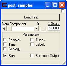
The control panel of post_samples is shown in the figure above.

The Load File button opens a File Browser which lists the *.apdv, *.aidv, *.geo, *.pgf or *.gmf files that are present in the current directory shown in the directory window.

To display nonvertical boreholes, the only requirement is that samples from any given borehole have the same location name, with the actual coordinates of each sampling location. The Data Component slider allows the user to select which of the property values in a file will be displayed by post_samples. For example, when reading CPT data the user may choose either tip resistance, sleeve friction or friction ratio using the slider. When reading contaminant data the user may choose among the various contaminants listed in the file. The default value is 0, which selects the first value that is present in the file. When reading .geo files, the data for all of the geologic layer tops will be read and displayed.

The Z Scale field displays the current Z exaggeration factor.

The Run toggle is used to turn on and off automatic execution of the module whenever a parameter is changed or a connection is made.

The Suppress Output toggle is used to prevent messages from the post_samples module from appearing in the Command Console.

Module Parameter Subpanels:

The post_samples module has five subpanels. These allow the user to:

set the parameters used while processing the input data
to specify the characteristics of the tube used to represent geology
to control how time data is displayed
to control the display of tubes, lines, colored tubes
to specify the types of labeling that will be displayed.

Clicking on the check boxes next to the subpanel names will bring up the subpanel parameter screens.

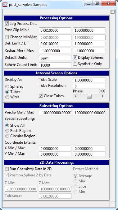
The Samples subpanel is shown in the figure above. It is important to note that all data processing actions are applied directly to the data in memory, and that the original data file is not altered. The data processing within post_samples applies only to the Sample indicators or tube coloring in the display. When setting data processing parameters in post_samples, the user should refer back to the preprocessing and/or postprocessing parameters set in any other modules that will contribute to the final display to assure that consistent parameters are being used (i.e., to correctly specify whether the data has been log transformed, scaled, and/or clipped). This is particularly important when a color scale is being used to display parameter value distributions on a 2D or 3D subset and spheres in the same display.

Processing:

The number entered into the Post Clip Min input field will be used after data processing to replace any sample property value that is less than the specified number.
- The default value for Clip Min is 0.001 when the Log Process Data toggle is on (default), but reverts to -1.0+e9 when it is off. The number entered into the
Post Clip Max input field will be used after processing to replace any nodal property value that is greater than the specified number.
- The default value for Clip Max is 1.0+e9 (so it won’t clip anything), but the user can enter any number less than your data maximum.

Notes:

The above CLIP values do change your data and how it will be displayed and labeled.
Setting the clip max outside your data maximum will not shift the data mapping outside your data range. If duplicate data values exist in files (data points with exact X, Y, and Z coordinates), these values are averaged to produce one data point for each unique coordinate.
If the log10 of the data is taken, the Clip Min value must be used to replace any zero values in the data with a specified Clip Min value that is greater than zero, to eliminate possible errors associated with attempting to take the log of 0 or negative number (which is undefined). The Log Process Data toggle is used to indicate that the log10 of the data read from the file is to be used.

The ChangeMin/Max toggle (and associated min and max type-ins) behave like the change_minmax module and sets the min and max values that are used by the datamap. This affects colors, but does not affect the actual data.
The Radius Min / Max input fields are used to specify the minimum and maximum radii of the spheres (or other sample indicators in user units), that will be used to scale the sample indicators to the value of the property being represented. If these values are set to zero the scaling procedure considers the extent in X-Y of the domain of the file being read by post_samples, to produce sample indicators that are easily seen on the display. When posting geophysical logs or CPT logs (with apdv files), the Radius Min / Max are commonly adjusted to different values to display the relative magnitude of the deflections along the borehole trace.
The Default Units field indicates in which units the data are to be considered if not specified in file.
The Sphere Count Limit field determines the maximum number of spheres to create. If the number of samples (spheres to be generated) exceeds this value, the module will turn spheres off and generate (more efficient) colored tubes instead.

Interval Screen Options:

The Display As radio box controls how the well screens will be displayed. If the Spheres option is selected, spheres are evenly distributed through the well screen based off the Max Gap parameter in the AIDV data file. If Tubes is selected the well screen will be displayed as a tube from the top of the well screen to the bottom. If Wires is selected the well screen will be displayed as a line from the top of the well screen to the bottom.
The Tube Scale field allows the user to input a value to scale the radius of the well screen tube by.
The Tube Resolution field changes the number of divisions used to make each well screen tube. The higher the resolution the smother or more circular each tube will be.
The Close Tubes toggle if turned on will place a disc, of the same resolution as the tube, inside the top and bottom of the tube. This gives the well screen tubes a more solid visualization.
The Phase slider will rotate the tube about its axis. This is more useful when using tubes of low resolution (e.g. flat-2 or triangular 3)

Subsetting Options:

The PreClip Min and PreClip Max fields allow you to view a subset of your data samples based on the numbers entered. The default value for Clip Min is -1.00e9, and for PreClip Max it is 1.00e9.
The purpose of Spatial Subsetting is to eliminate samples from being processed. This can be accomplished in two ways. The first is by connecting a surface to the subset surface port of the module (in EVS PRO and MVS), this can eliminate all samples within, or outside of the boundaries of the surface. The second is to define the type of region and extents of the region you wish to include in the processing. This eliminates all samples that fall out of the defined area.

$image\postsamples_rectsub.jpg$

To subset by a rectangular region the XY extents of the region must be defined.

$image\postsamples_circsub.jpg$

To subset by a circular region the XY center of the circle must be defined as well as the radius.

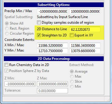
The Cut inside surface toggle is used when a surface is input to the 4th input port. This toggle, when OFF gives you all borings inside of the surface. When ON gives you all samples outside of the surface.

The Straighten to 2D toggle shown above is used to project your 3D borings to a 2D representation. It creates a subset of your data which falls within the Distance to Line distance from a line segment input to the 4th input port. This functionality is typically used in conjunction with the related 2D straightening in the thin_fence module. You would use the same line input as you're using on thin_fence in that case.

The Export in XY toggle projects the data onto the XY plane vs. the XZ plane. This is the more useful option if the results are to be used in ESRI's ArcMAP.

Please note that the coordinate extents of straightened borings will be to the right of the origin (0,0). It is best to create 2D projections in a separate Viewer from any other objects in your application.

The Coordinate Extents are read only and are there for reference when defining your subset area.

2D Data Processing:

Checking the Run analyte (e.g. chemistry) Data in 2D toggle will cause any 3D data you have to be turned into 2D data based upon the Extract Method.

The 3D->2D subsetting will use the same rules and methods used by Krig_2D, so that the results from post_samples will show the actual values which Krig_2D would use internally in the kriging process.
Any values in your data entered as "<x.xx" will be multiplied by the current LT (multiplier) and the resultant value will be used for all subsetting operations.

There are four different types of extraction methods.

The first, Average, will take the average data values for all samples sharing an (X,Y) coordinate, it will then place one sample with that average at the (X,Y) location.
The second method,Max, will take the maximum value for all samples sharing an (X,Y) location and then place a sample with that value at that (X,Y) location.
The third method, Slice allows the user to select a z coordinate for the slice position as shown below. It will then find the closest samples to that z location that share (X,Y) coordinates. If there is a sample at that exact location, it will use the data from that sample to create a point at that (X,Y) location. If it is between two samples it will interpolate the data between them based on their distance from the slice position. It will use that interpolated data to create a new point.
The final method, Min, will take the minimum value for all samples sharing an (X,Y) location and then place a sample with that value at that (X,Y) location.

The Position Sphere Z by Data toggle will set the Z component of the sphere to the value of the first data component.

$image\postsamples_geology.jpg$

GeologyPanel

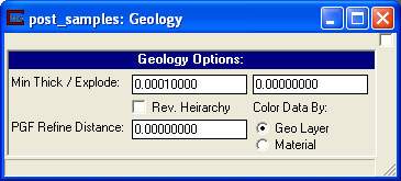
The Geology is useful when reading in a geology based file (*.geo, *.pgf, *.gmf).

The Min Thickness is the smallest thickness, in user coordinate units, that a geological layer can have.

The Explode(EVS PRO and MVS Only) distance can be set here or referenced by connection from the Explode_and_Scale module. NOTE: For *.geo files, the samples will be exploded based upon their layer designations unless a different geology is imported into the module.

The Rev. Hierarchy toggle will reverse the hierarchy of the geology. Normal hierarchy will push down any layer that tries to rise through the one above it. Reverse hierarchy will pull up any layer that dips into the one below it.

The PGF Refine Distance is used when pgf files are displayed as spheres. At minimum there is a sphere at the top and bottom of each layer, the refine distance will add spheres between those two spheres until no sphere is more than the refine distance apart.

The Color Data By radio box will color the sample spheres by either the Geological layer or the Material value of that layer.

$image\postsamples_time.jpg$

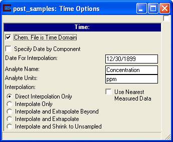
Time Panel

(EVS PRO and MVS Only)

This panel is for analyte (e.g. chemistry) files (*.apdv, *.aidv) that are set up as time domain files (i.e. one analyte whose values are recorded over time).

The Chem. File is Time Domain toggle turns on date interpolation for time domain analyte (e.g. chemistry) files.

The Specify Date by Component toggle will cause the Date for Interpolation field to be ignored and the date to be selected using the component slider.

The Datefor Interpolation field is the date being interpolated to, for example if you have an analyte value of 2 on 1/01/05 and a value of 4 on 1/03/05 and the date is set to 1/02/05 with Direct Interpolation the value should be set to 3. The Date can be either set by hand or imported. This makes the module useful in a time_loop.

In time domain files there is no place to set either the analyte name that has been kriged over time or the analyte units; these can be set in the Analyte Name and Analyte Units fields.

The Use Nearest Measured Data toggle causes the sample at the interpolated date, to have the same value as the nearest measured date

There are 5 different Interpolation methods that are available, each interpolation method is used to define how to interpolate when given non-detects in a file.

Direct Interpolation Only: This is the most basic interpolation method, and the most accurate in terms of representing the data as it has been entered. This method looks at the two dates surrounding the input Date. If either date, or both dates, have non-detects as values, the value for that sample will be a non-detect and no interpolation will occur. If neither date has a non-detect value it will interpolate between them.
Interpolate Only: This method will look at the two dates surrounding the input Date. If the date before the input Date is a non-detect it will continue to look backwards through each time column until it finds a date with a value that is not a non-detect. If the date after the input Date is a non-detect I will look forward through the time columns until it finds a date that is not a non-detect. If either search fails to find a useable dates then it will set the value for that time to a non-detect value. Else it will interpolate between the two found dates. This is useful for files that have a small amount of non-detects.
Interpolate and Extrapolate Beyond: This method will look at the two dates surrounding the input Date. If the date before the input Date is a non-detect it will continue to look backwards through each time column until it finds a date with a value that is not a non-detect. If the date after the input Date is a non-detect I will look forward through the time columns until it finds a date that is not a non-detect. If it does not find a date with a non-detect after the input Date, it will extrapolate beyond the last useable date to the input Date.
Interpolate and Extrapolate: This method will look at the two dates surrounding the input Date. If the date before the input Date is a non-detect it will continue to look backwards through each time column until it finds a date with a value that is not a non-detect. If it fails to find one it will extrapolate the first value backwards to the input Date. If the date after the input Date is a non-detect I will look forward through the time columns until it finds a date that is not a non-detect. It will also extrapolate beyond the last valid date in the file.
Interpolate and Shrink to Non-Detect: This method will look at the two dates surrounding the input Date. It will shrink the size of the sphere when interpolating to a non-detect from a valid value, and will grow the size of the sample sphere when interpolating to a valid value from a non-detect. If the Non-Linear Shrink toggle is selected the size of the sphere will be determined by a cosine interpolation instead of a linear one. In the case of interpolating to a non-detect from a valid value, this causes the size of the sphere to shrink very slowly at first and then to shrink more quickly as the date approaches the non-detect date.

$image\postsamples_tubes.jpg$

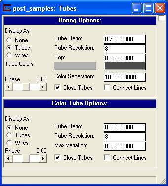
Tubes panel

The Tubes panel, shown above, handles the options for boring tubes and for creating color tubes. Both of these tube types are based on the boring ID’s in a file. However, the Boring tubes will rise all the way to either the value in the Top field or the Top value specified in the file, while the Color Tubes will start at the highest sample location for each boring.

Boring Options

The Display As radio box change how the Boring tube is displayed, you can either turn off the tube entirely, display it as a tube, or display it as a wire.

The Tube Ratio field is a double value between 0.0 and 1.0 that sets what percentage of the sample sphere minimum radius the tube radius will be. For example if you have sample spheres with a minimum radius of 10 and the Tube ratio is set to .7, then the radius of each tube will be 7.

The Tube Resolution indicates how many faces will be used to create each tube; increasing this number will result in rounder tubes, but will use more memory. The minimum value for this field is 2 which creates plane like tubes, 3 will create triangular shaped tubes, 4 will be square, etc...

The Top value will set top elevation for each tube. If this value has been specified in the file, the file value will be used instead of this value.

Tubes are broken up into cells of two colors to help give a visual clue as to scale. These colors can be set by using the Tube Colors buttons. The height of each cell can be set using the Color Separation field. NOTE: Having a small Color Separation on a large model can impact performance because of memory demands.

The Phase slider will rotate a tube about its axis.

To put a cap on the top and bottom of each Boring Tube check the Close Tubes toggle.

The Connect Lines toggle is used for non-vertical borings. The best way to visualize this function is to use an example of 3 non-vertical samples. A cell will be created between the first and second sample and another cell will be created between the second and third sample. Because these are necessarily separate cells the ends between the cells may not be coincident. This is especially evident when looking at borings with large changes in angle between samples, or kinks. To merge these cells into a single tube the separate ends are "averaged" causing a distorted, but more efficient and seamless tube.

Color Tube Options:

The functions of the Color Tubes match those functions of Boring Tubes with the same names. Where Boring Tubes are separated by two distinct bands of color for a visual scale clue, Color Tubes are colored by the nodal data component.

The Max Variation value is a tool used to correct color blending between samples. Color tubes is actually interpolating the color of the tube between two samples based upon the color of the spheres, not upon their data. For example, if one sphere has a value at your data max and is colored red and the next sphere in the boring has a value at your data min and is blue, it would color the tube at the midpoint between these spheres purple, a color which does not exist in the default datamap. By forcing new points to be generated between these, we can prevent these discolorations from occurring. A value of .33, the default, states that any samples which lie next to each other along the tube and whose data varies by more than 33% of the total data range will automatically get extra points inserted between them.

$image\postsamples_labels.jpg$

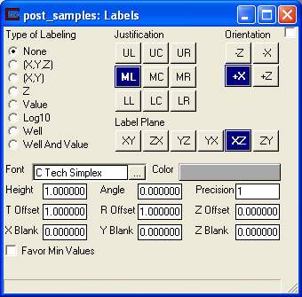
Labels panel

The Type of Labeling radio box will allow the user to select what to label for each sample

None - Do not label samples.
(X, Y, Z) - Label each sample with its x, y and z coordinates.
(X, Y) - Label each sample with its x and y coordinates.
- Label each sample with its z coordinates.
(Value) - Label each sample with its analyte value.
(Log10) - Label each sample with the log base 10 of its analyte value.
(Well) - Label the top of each well or boring with the well or boring id.
(Well And Value) - Label the top of each well or boring with the well or boring id, and label each sample with its value.

The Justification buttons define how the labels will be justified around the samples.

The Label Plane options determine in which plane to write the labels.

The Orientation buttons determine in which direction in the label plane to write the labels.

The Font for the labels is by default C Tech Simplex, which is a low memory type font. For a font that will always be facing the view regardless of rotation, switch to Forward Facing font.

The Color button will change the color of the labels.

The Height field will change the height of the labels.

The Angle field determines where in a circle around the sample to place the label. For example a value of zero means place the labels to the direct right of the sample, a value of 90 would place the label directly above the sample.

The Precision field indicates to what precision to display any float or double values being displayed as labels.

The T Offset field is the title (the well or boring ID label) offset in the z direction. This can raise or lower your title and is added to the Z offset to determine the z location of the title.

The R Offset field is the radial offset, this determines how far from the sample to place the label, a value of 1 means to add the radius of the sphere to the XYZ location of the sample and place the label there.

The Z Offset is added to the Z coordinate in labeled sample to raise or lower the labels in the Z direction.

The X Blank, Y Blank, and Z Blank fields create a 3D box that will allow only the label at the highest value to be displayed inside. If there are multiple samples with the same max value within the box, the label that is displayed is based upon the order processed, which is not necessarily the order defined in the file. The Favor Min Values toggle will switch this behavior to display the label at the minimum value.

Interactive Querying of Your Data

The post_samples module allows you to probe any sphere and determine information about that sample and its borehole ID. To probe a sample, first verify that you have spheres on, click on any sphere with Left Mouse Button while holding down the Alt key. The following window will appear in the upper right hand corner of your desktop.

$image\postsamples_probe.jpg$

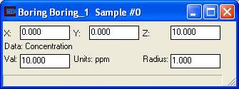
X (Easting)

Y (Northing)

Z (Elevation)

Data: (Current sample’s nodal data name)

Val: (Sample Value)

Units: (Sample Units)

Radius: (Sphere Radius)