

General Module Function
Krig_3D models three-dimensional parameter distributions within rectilinear domains defined by the limits of the data set, or by the convex hull, rectilinear, or finite-difference grid extents of a geologic system modeled by Krig_3D_Geology. It creates a hexahedral finite-element grid with kriged nodal values of any scalar property and its kriged confidence level, and outputs a geometry whose elements can be filtered, sliced and rendered to view the color scaled parameter distribution on the element surfaces and/or edges. Krig_3D provides several convenient options for pre- and post-processing the input parameter values, and allows the user to consider anisotropy in the medium containing the property.
Krig_3D has the ability for this module to create uniform fields, and the ability to choose which data components you want to include in the output. There are a couple significant requirements for uniform fields. First, there cannot be geologic input (otherwise the cells could not be rectangular blocks). Second, Adaptive_Gridding must be turned off (otherwise the connectivity is not implicit).
Module Input Ports
input0 (Blue/Grey/Green): This port can accept a data field from Krig_3D_Geology to krig data into geologic layers. Please note that if any portions of the input geology is NULL, these cells will be omitted from the grid that is created. This can save memory and provide a means to cut (in a Lego fashion) along boundaries
External_Grid (Blue/Black): (Available only in MVS) This port (blue/black) allows the user to import a previously created grid. All data will be kriged to this grid.
Read__data_file (Yellow/Blue/Yellow): This port allows the sharing of file names between similar modules.
External_Data (Blue/Black): (Available only in MVS) This port allows the user to import a field contain data. This data will be kriged to the grid instead of using file data..
Module Output Ports
Read__data_file (Yellow/Blue/Yellow): This port allows the sharing of file names between similar modules.
status_out (Blue-Green) : This port outputs a string that has the current status message from the module. This string is updated as the module runs.
Sphere_Out (Red): This port outputs a renderable sphere to the view, this sphere represents the location of maximum uncertainty.
Out1 (Blue/Black): This port outputs a 3D data field which can be input to any of the Subsetting and Processing modules which have the same color port
![]()
When the Plot Semivariogram option is selected three additional output ports will appear as in the above figure.
Out2 (Red/Grey): This port outputs a renderable geometry of the calculated semivariogram.
VG_fld_out(Blue/Black): This port outputs a 3D data field representing the lines (semivariogram cloud pairs) and is provided primarily for connection to the axes module.
VG_scale_fact (Grey/Brown): This port is the Z_Scale of the semivariogram plot and is also provided primarily for connection to the axes module.
Module Control Panel
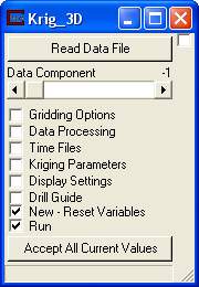
The control panel of Krig_3D is shown in the figure above.
The Read Data File button opens a File Browser as described for Krig_3D_Geology, but which lists the *.apdv;*.aidv; or*.vdf files that are present in the current directory shown in the directory window. The format of .apdv files is described in the apdv_file_format help topic.
Note that this module will not begin running until a valid analyte (e.g. chemistry) file has been selected, or a valid field containing data has been imported, and the Accept All Current Values button is pushed.
The Data Component slider allows the user to select which of the property values in the analyte (e.g. chemistry) file will be kriged by execution of the module. The default value is -1, which results in kriging of all of the data components in the file during a single execution of the module.
The "Run" toggle controls whether the module will run when applications are loaded or data changes. When this is on, the module runs when applications are loaded or the "Accept" button is pushed (or the geology input changes). When it is off, the module will not run.
The "New-Reset Variables" toggle (on by default) resets all expert system calculated variables to zero before each run. This allows multiple calculations to be performed without tedious manual resetting of these variables. To change an expert system calculated variable, the toggle must be off.
Module Parameter Subpanels
Krig_3D has six subpanels which allow the user to set the parameters used for preprocessing the input data, producing the semivariogram, executing kriging, and post processing kriged output. Clicking on either the check boxes next to the subpanel names, or on the names themselves will bring up the subpanel parameter screens.
Module Status: Interruptible
This module's computational processes can be terminated (interrupted) using the "C Tech" icon in the Windows Notification Area (aka System Tray) in the lower right corner of your desktop. If you hover over the icon, it will tell you the status of the module and expected completion time. Double-Right-Clicking will terminate the process. Note that if you do stop any process, the output of the module is corrupted and any downstream module's results are not usable. You will need to re-run the module.

Gridding Options
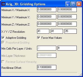
The Gridding Options subpanel is shown in the figure above. It is used to specify all parameters that affect the grid exported from Krig_3D. The availability of many options depends on whether geologic input is available or if the grid is created totally within Krig_3D. The window above shows the options with no geologic input. NOTE: If an external grid is imported into Krig_3D this panel will be blank.
The Minimum X, Maximum X, Minimum Y, Maximum Y, Minimum Z and Maximum Z parameters allow the user to define the horizontal and vertical domain within the data set in which kriging of the parameter distribution will be completed. A value of 0 is the default for these parameters, which results in a model domain that is defined by the rectilinear bounds of the entire data set when the module is run. Krig_3D utilizes a model domain that is bounded by the limits of the data set, unless the user specifies a different domain by setting the Min and Max Values for X, Y, and Z, or it is passed a model (or finite-difference) domain from Krig_3D_Geology. Utilizing the default extents effectively minimizes the extrapolation of parameters within the model to that area which is enclosed by the measured data points. Note that when a geologic model domain is passed to Krig_3D, the kriging domain is restricted to that domain regardless of what X, Y, or Z values are set in the Krig_3D inputs. The geologic model domain can be bounded by the convex hull of the data set, or by some specified offset (see discussion in Krig_3D_Geology). If the user is uncertain of the X, Y and Z limits of the data domain, the module should be run with the default 0 values, and upon completion of execution, the values in the X, Y, and Z input fields will be the min and max values of these parameters in the data set. The File_Statistics module can also be used to investigate the limits and distribution of values in the input data set, and the statistics module can be used to output the distribution of values in the kriged model.
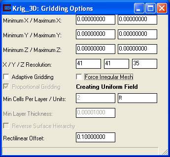
Krig_3D has the ability for this module to create uniform fields, and the ability to choose which data components you want to include in the output. There are a couple significant requirements for uniform fields. First, there cannot be geologic input (otherwise the cells could not be rectangular blocks). Second, Adaptive_Gridding must be turned off (otherwise the connectivity is not implicit). Finally, when both of these conditions are satisfied, you turn off the toggle "Force Irregular Mesh", which is on by default (as shown below). This results in the output field being a uniform field. Uniform fields are more memory efficient and allow the use of several "field" specific modules like: orthoslice. They also have the ability to use the volume_renderer directly on the output!
The X / Y / Z Resolution parameters specify the number of grid nodes that will be included within the model domain. If Indicator_Geology is being passed a model domain from Krig_3D_Geology, then the x-y values are not used . The number of grid elements along any axis of the model is simply the axis Res value minus one, as every element has two bounding nodes along an axis. The default value for the X and Y Res parameters is 41, and the default value for the Z Res is 35. [note: these values were increased substantially as of version 6.0 in response to ever increasing computer speeds] However, the user can specify any number desired, up to the limit of available memory resources in the computer and run time limitations imposed by the patience of the user.
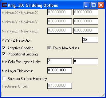
If geologic layers are being passed to Krig_3D, then the number of nodes specified in Z Res will be distributed over the geologic layers in a manner that is approximately proportional to the fractional thickness of each layer relative to the total thickness of the geologic domain.
NOTE: If Proportional Gridding is toggled off then only Min Cells per Layer is enabled. In this case, only the Min Cells per Layer input will be used for each layer of the model.
The Adaptive Grid toggle refines the grid automatically to place grid nodes at all of the measured data points. The adaptive grid will result in a kriged parameter distribution that honors all of the measured data points exactly. This is the default domain used by Krig_3D. EVS PRO's improved Adaptive Gridding uses the following options and logic. It will perform grid refinement on any cell containing one or more samples and when there is more than one sample it will (usually) refine the two samples having the highest and lowest values. This assures that your kriged grid will always honor the total range of your data and ensures that data where low values are most important (e.g. pH) are handled optimally.
Proportional Gridding - A toggle for activating the same algorithm for apportioning nodes in the Z direction as used in Krig_3D. The number of nodes specified for the Z Resolution will be distributed (proportionately) over the geologic layers in a manner that is approximately proportional to the fractional thickness of each layer relative to the total thickness of the geologic domain. In this case, at least three layers of nodes (2 layers of elements) of the Krig_3D domain will be placed in each geologic layer.
Min Cells per layer - A Type in for establishing a minimum number of cells (in the Z direction) per layer. The default is 2 cells which results in 3 nodes.
Units – This field contains the default coordinate units for the grid, if no coordinate units are specified in the file being read, these units will be used.
Reverse Surface Hierarchy – This toggle determines whether the surfaces will define layers in a normal (top to bottom) manner or reversed (if on). This topic is discussed in more detail in Workbook 12.
The Rectilinear Offset parameter is used to create an automatically generated rectilinear domain which is larger than the input data set by a user input percentage along all three axes. If 10% (0.1 default value) is used, the limits will be offset by 5% on all 6 sides of the rectilinear volume.
Data Processing
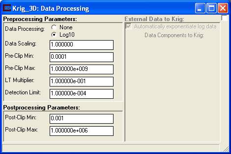
The Data Processing parameters subpanel is shown in the figure above. It is divided into three groups which are Preprocessing. Postprocessing, and External Data to Krig.
It is important to note that all preprocessing actions are applied directly to the data in memory, and that the original data file is not altered. However, all of the functions within Krig_3D and the modules downstream of Krig_3D will be using the preprocessed (and kriged) parameter distribution. The user should refer back to the preprocessing subpanel when setting values for the filtering and display of the kriged data (i.e., to correctly specify whether the data has been log transformed, scaled, and/or clipped).
The Data Processing radio buttons allow the user to specify whether the data will be used as is, or will be processed to compute the log (base 10) of the parameter value before kriging. Note that if the log10 of the data is taken, a Clip Min value (which must be greater than 0) must be used to replace values in the data below the specified minimum value because the log function is undefined for values equal or less than zero.
The Data Scaling input field is used to specify a value by which all nodal data values will be multiplied before kriging. The default value is 1, but the user can specify any negative or positive value. This option is most commonly used to convert the units of the property being kriged, such as to convert concentrations in ppb to ppm or visa-versa. The user should bear in mind that any scaling of the data that is completed in Krig_3D will affect all downstream modules, which is especially important when using the Volume and Mass module downstream of Krig_3D.
The number entered into the Pre-Clip Min input field will be used during preprocessing to replace any nodal property value that is less than the specified number. When log processing is being used, the value of Clip Min must be a positive, non-zero value. Generally, Clip Min should be set to a value that is one-half to one-tenth of the lowest detection limit in the data set, unless the user wishes to make the influence of not detected values stronger. As an example, if the lowest detection limit is 0.1 (which is present in the data set as a 0), and the user sets Clip Min to 0.0001, the clipped non-detected values forces three orders of magnitude to be present between any detected value and the non-detected values.
The number entered into the Pre-Clip Max input field will be used during preprocessing to replace any nodal property value that is greater than the specified number. The clipping values can be used to lessen the importance placed on extremes of the data, or outlier data values, before kriging. The preprocessing functions can be used in various ways to investigate the kriging confidence levels within specified ranges or limits of the data sets. An example of this type of analysis is provided in the Sample Networks section.
The LT Multiplier value affects any file value with a preceeding "<" character. It will multiply these values by the set value.
The Detection Limit value affects any file values set with the "ND" or other non-detect flags (for a list of these flags open the help for the APDV file format). When the module encounters this flag in the file it will insert the a value equal to (Detection Limit * LT Multiplier).
Postprocessing of the data from Krig_3D affects the calculation of the kriging confidence and uncertainty estimates that are produced by the model, and allows the user to apply a filter for the data passed to all modules downstream of Krig_3D. Note that the postprocessing does not affect any of the other Semivariogram or kriging algorithms that execute in Krig_3D, so the user can experiment with different values of postprocessing parameters to obtain the type of display desired, independent of the internal kriging process.
The Post-Clip Min parameter specifies the smallest nodal value that will be present in the data field output by Krig_3D. This parameter is useful for limiting or enhancing the effects of not detected values or outliers in a data set, and for optimizing the use of the dynamic color range used to represent the property distribution. Clip Min has a default value of 0.001, but can be set to any negative or positive value with magnitudes from -1.0 E09 to 1.0 E09. In general, good results are obtained by setting this value to the lowest property value or detection limit in the input data set. It is important to note that because not detected values are represented in the .apdv file as zeros, the Clip Min value can be used to strengthen the influence of small values or non-detects that are present in the data set. As an example, if the detection limit for a certain chemical analysis is 0.1 (which is entered into the .apdv file as 0), and the Clip Min is set to 0.0001, then this not detected value will have an effective influence on the kriged distribution near this data point that is three orders of magnitude stronger than the actual detection limit. The user should bear in mind that if mass or volume estimates are being made in the analysis, the Clip Min value could affect the estimates if considerable data are present that are being clipped. For volume estimates, if the specified lower bound of the concentrations of interest is well above the Clip Min value, then their will be no effects on the results. If the specified lower bound of concentrations for the volume estimate is lower than Clip Min, then the clipping will truncate the volume at the Clip Min value, and the estimated volume will be from the entire model domain.
The Post-Clip Max parameter specifies the largest nodal value that will be present in the data field output by Krig_3D. Again this parameter can be used to optimize the use of the dynamic color range when a data set has a few extremely high values, but the user is most interested in seeing the detailed changes in the distribution in some lower range of the data. It can also be used to investigate the kriging confidence or uncertainty levels near certain threshold values of a property. As an example, if the regulatory threshold for a parameter is 10 units, then the Clip Max parameter can be set to 10, and all kriged values greater than 10 will have the same strength in the calculation of the uncertainty levels in the kriged distribution. Clip Max has a default value of 1,000,000, but can be set to any negative or positive value with magnitude form -1.00E09 to 1.00E09.

When external data is being imported into the module the External Data to Krig window becomes active. This window allows the user to select which data components to krige by switching on or off the toggles associated with that data component. The Automatically exponentiate log data toggle will detect if the data being imported has been log processed and if it has exponentiate it. This avoids double log processing the data with the Preprocessing option.
Time Files
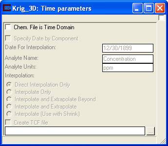
(EVS PRO and MVS Only)
This panel is for analyte (e.g. chemistry) files (*.apdv, *.aidv) that are set up as time domain files (i.e. one analyte whose values are recorded over time).
The Chem. File is Time Domain toggle turns on date interpolation for time domain analyte (e.g. chemistry) files.
The Specify Dateby component toggle causes the module to ignore the user specifed date and instead use the component slider to select the date.
The Date for interpolation field is the date being interpolated to, for example if you have an analyte value of 2 on 1/01/05 and a value of 4 on 1/03/05 and the date is set to 1/02/05 with Direct Interpolation the value should be set to 3. The Date can be either set by hand or imported. This makes the module useful in a time loop.
In time domain files there is no place to set either the analyte name that has been kriged over time or the analyte units; these can be set in the Analyte Name and Analyte Units fields.
There are 5 different Interpolation methods that are available, each interpolation method is used to define how to interpolate when given unsampled times in a file.
Direct Interpolation Only: This is the most basic interpolation method, and the most accurate in terms of representing the data as it has been entered. This method looks at the two dates surrounding the input Date. If either date is unsampled, the value for that sample will remain unsampled and no interpolation will occur. If both dates have sampled values it will interpolate between them.
Interpolate Only: This method will look at the two dates surrounding the input Date. If the date before the input Date is an unsampled date it will continue to look backwards through each time column until it finds a sampled date.. If the date after the input Date is unsampled it will look forward through the time columns until it finds a sampled date. If either search fails to find a useable dates then it will set the value for that time to a unsampled value. Else it will interpolate between the two found dates. This is useful for files that have a small amount of unsampled values.
Interpolate and Extrapolate Beyond: This method will look at the two dates surrounding the input Date. If the date before the input Date is an unsampled date it will continue to look backwards through each time column until it finds a sampled date. If the date after the input Date is unsampled it will look forward through the time columns until it finds a sampled date. If it does not find a sampled date after the input Date, it will extrapolate beyond the last useable date to the input Date.
Interpolate and Extrapolate: This method will look at the two dates surrounding the input Date. If the date before the input Date is an unsampled date it will continue to look backwards through each time column until it finds a sampled date. If it fails to find one it will extrapolate the first value backwards to the input Date. If the date after the input Date is unsampled it will look forward through the time columns until it finds a sampled date. It will also extrapolate beyond the last valid date in the file.
Interpolate(Use with Shrink): This method uses the same interpolation method algorithm as Direct Interpolation. It is used for clarity when there is a post_samples or file_statistics module in the network that is using the Interpolate and Shrink to Unsampled option on the same file.
The Create TCF File toggle will cause the Krig_3D module to run in a loop, going through each component and creating an EFB file at that time. These EFB files will be linked together in the specified TCF file and can be used with the Read_TCF module for animation purposes. NOTE: This function will not work unless a TCF name is selected as well.
Kriging Parameters
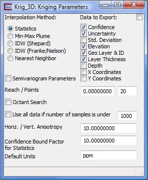
The Kriging Parameters subpanel of Krig_3D is shown in the figure above.
The Interpolation Method radio buttons determine:
The type of statistical information which will be included in the nodal data components (statistics vs Min-Max Plume option)
IDW Shepard
IDW Franke/Nielson
Nearest Neighbor.
If Statistics is chosen, Each Concentration (for every chemical in the .apdv file) will have a corresponding Confidence (based on the Confidence Bound parameter) and Uncertainty. The display when Statistics is selected and the data is log processed is shown above.
The display when Statistics is selected and the data is NOT log processed is shown below. In this case, the confidence bound is a tolerance vs. a factor.
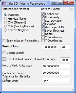
If Min-Max Plume is chosen three different Concentration components will be calculated, the Nominal, Minimum and Maximum. These different distributions are determined based on the standard deviation and nominal concentration at each node based on the Confidence parameter which is expressed in percent (nominally 60%). Note that at a "confidence" of 50%, the nominal, minimum and maximum concentrations are identical.
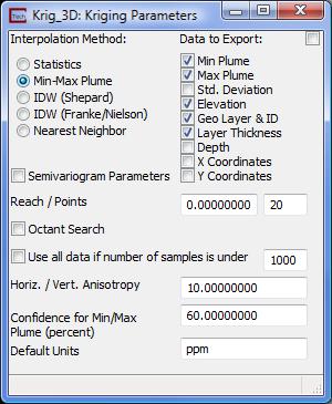
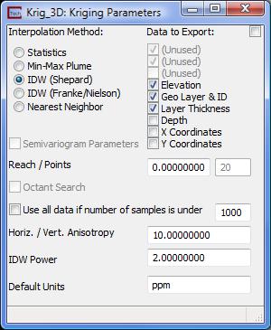
If either Inverse Distance Weighted (IDW)estimation method (Shepard and Franke/Nielson) is selected, kriging is not performed and one of these algorithms is used as an alternative to kriging in Krig_3D. This also affects the available parameters as show in the figure below:
Note: The "new" toggle on the main panel (on by default) resets all expert system calculated variables to zero before each run. This allows multiple calculations to be performed without tedious manual resetting of these variables. To change an expert system calculated variable, the toggle must be off.
The Reach input field defines the radial distance (in user units) from any given model node that the kriging module will look for data points to be included in the estimation of the model parameter at that node. The default value of reach is 0, which results in the module calculating a reach value which is approximately two-thirds of the longest distance between any two data points in the data set.
NOTE: If your Reach value is set so small that for some points in your grid, no samples fall within the Reach ellipsoid (it is a sphere distorted by the Horizontal/Vertical Anisotropy), you can receive an error message that will abort the kriging process. The error is Matrix Singular in one or more areas. This is unlikely to occur if you do not reset the Reach unless you set an extremely high Horizontal/Vertical Anisotropy. Highly clustered data with large regions without sampling can cause this to occur.
The only solutions are to increase Reach, reduce Horizontal/Vertical Anisotropy (if that is suspected) or revise the extent of your model in x-y and/or z.
The Points parameter defines the maximum number of data points (within the specified reach) that will be considered for the parameter estimation at a model node. The default value for points is 20, which generally provides reasonably smooth modeled parameter distributions. The effects of decreasing and increasing the values for reach and points on the model output are somewhat similar, but for different reasons. If the data have a fairly even spatial distribution throughout the domain, then increasing these values will generally include more of the input data points that will be used to krige the value for a given model node, and thus will result in smoother modeled data distributions. Decreasing the values of reach and points (in an evenly distributed data set) results in fewer input data points being used to calculate the parameter estimates at a given model node, and result in modeled distributions with greater variations across smaller areas.
The user should consider both the spatial distribution and the range of values in the input data set when deciding upon values for the reach and points parameters. If the specified reach is too small to allow the kriging module to locate at least one point within the search area, then no kriging can be done and the module will terminate with an error message..
If the user specifies a large number of points (that are within the specified reach), then the output will be smoother, but the execution time for the kriging can sometimes increase significantly. By posting the input data using the post_samples module, and looking at the characteristics of the resulting kriged data using the statistics module, the user can quickly analyze the characteristics and distribution of the kriging output for a given set of parameters, and test the effects of changing the kriging parameter values.
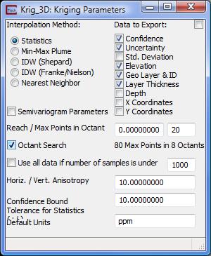
The Octant Search toggle changes the method by which data sample points are selected for inclusion in the kriging matrix. If this is on, the "Points" parameter switches to "Max Points in Octant". Searching is performed for each of the eight Octants surrounding the point to be kriged. Within each octant a maximum number of points (up to one-fourth of the total points) are selected. Then, points are taken sequentially from each octant up to the maximum number of total points or until all octant's points have been used. The panel display changes when this option is selected as shown above. Octant Search is applicable for the Statistics and Min-Max Plume kriging modes.
The type-in value for Use all data if number of samples is underis off by default, but this option gives the smoothest plumes since all data is used for the kriging process. Sometimes using all points results in faster computation since only one (large) kriging matrix must be solved.
The Horiz./Vert. Anisotropy Ratio parameter allows the user to consider the effects of anisotropy in the conductivity of soil matrices to fluid flow. In most cases, geologic materials are deposited with platy clay minerals oriented horizontally, and thus flow of water in both the saturated and unsaturated zone can be slower in the vertical direction than in the horizontal direction. Also, ore deposition can occur along horizontal or vertical fault or fracture systems. Chemical constituents being transported with flowing fluids may therefore show a larger degree of spreading in one or the other direction. The Horiz./Vert. Anisotropy Ratio basically tells the kriging algorithm what multiplication factor should be used to apply biased weighting on data points in horizontal and vertical directions away from a given model node. The default value is 10, which allows data points in a horizontal direction away from a model node to influence the kriged value at that node 10 times more than data points an equal distance away in a vertical direction. However, the user can specify any positive number with a magnitude up to 100,000. When the property being modeled is not related to fluid flow or other processes that might be affected by matrix anisotropy, then this parameter should be set to 1.
The Confidence Bound parameter is used to specify what interval around the kriged model estimates the kriging confidence or uncertainty will apply to. The default value is 10, which essentially produces the confidence and uncertainty that the kriged data are within one order of magnitude of the "true" value. As an example, if the Confidence Bound is 10, the kriged property value at a node is 5, and the kriged confidence level at the node is 0.9, then 90% of the time, the "true" value of the kriged property at that node will be in the range of from 0.5 to 50 units. Additional discussions of confidence and uncertainty are provided in the Sample Networks.
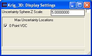
The Display Settings window is shown in the image above. This window controls the display of the uncertainty sphere location. By default there is one uncertainty sphere for every analyte. The visibility of the spheres can be toggled on and off by click on the check box next to the name of the analyte. These spheres can also be vertically exaggerated to match any downstream scaling of the field itself.
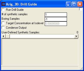
The DrillGuide© panels is shown above. When the Run Drill Guide toggle is selected Krig_3D will run in a loop creating a synthetic boring at the maximum uncertainty location until it has reached the set # of synthetic samples.
The Boring Samples field indicates how many samples create at each synthetic boring that is created.
The Target Concentration at subsetting level toggle, when selected, changes the location of the uncertainty sphere based upon the specified target concentration.
The Condense Output toggle, when selected, will minimize the number of strings displayed in the EVS console window.
The User-Defined Synthetic Samples slider is used to add points to the grid for drill guide purposes. The purpose of this slider is to help eliminate areas of high uncertainty that cannot be drilled, for example under a building.
Krig_3D Module Hints
Manually adjusting kriging parameters
The user must uncheck the new toggle in the main window in order to make manual adjustments to most parameters in this module. Otherwise the values will be calculated by EVS according to the spatial extents or distribution of the data.
© 1994-2018 ctech.com